DATA_SECTION

!! ad_comm::change_datafile_name("surp_prod1.dat");
 init_int fyear;
 init_int lyear;
 init_vector cat(fyear,lyear);
 init_vector cpue(fyear,lyear);


PARAMETER_SECTION

 init_number log_r;
 init_number log_q;
 init_number log_K;
 init_number log_sd_cpue;
 init_vector log_F(fyear,lyear);

 number r;
 number q;
 number K;
 number sd_cat;
 number sd_cpue;

 vector bio(fyear,lyear+1);
 vector cat_hat(fyear,lyear);
 vector cpue_hat(fyear,lyear);
 vector expl_out(fyear,lyear);
 vector F(fyear,lyear);

 objective_function_value jnll;


INITIALIZATION_SECTION

 log_r -0.6
 log_q -1
 log_K 8.5
 log_sd_cpue -1
 log_F 1


PROCEDURE_SECTION

 int t;
 dvariable expl;

 // Convert from log to normal space
 r = mfexp(log_r);
 q = mfexp(log_q);
 K = mfexp(log_K);
 F = mfexp(log_F);
 sd_cat = 0.05;
 sd_cpue = mfexp(log_sd_cpue);

 // Project the model forward
 bio(fyear) = K;
 for (t=fyear; t<=lyear; t++) {
   expl = 1.0/(1.0+F(t));
   bio(t+1) = bio(t) + r*bio(t)*(1.0-bio(t)/K) - expl*bio(t);
   cat_hat(t) = expl * bio(t);
   expl_out(t) = expl;
   cpue_hat(t) = q * bio(t);
  }

 // Compute the likelihoods
 jnll = 0;
 for (t=fyear; t<=lyear; t++) {
  jnll += 0.5 * square(log(cat(t)/cat_hat(t)) / sd_cat) + log(sd_cat);
  jnll += 0.5 * square(log(cpue(t)/cpue_hat(t)) / sd_cpue) + log(sd_cpue);
 }


GLOBALS_SECTION

  #include <admodel.h>
  #include <admb2r.cpp>


REPORT_SECTION
 open_r_file("out.rdat", 6, -999);
  wrt_r_complete_vector("obs_cat", cat);
  wrt_r_complete_vector("obs_cpue", cpue);
  wrt_r_complete_vector("est_bio", bio);
  wrt_r_complete_vector("est_cat", cat_hat);
  wrt_r_complete_vector("est_cpue", cpue_hat);
  wrt_r_complete_vector("est_expl", expl_out);
  wrt_r_item("jnll", jnll);
 close_r_file();


FINAL_SECTION

  // extract Hessian matrix
  open_r_file("hessian.rdat");
    open_r_matrix("hessian");
      wrt_r_matrix(get_hessian(),1,1);
    close_r_matrix();
close_r_file();Jitter test in ADMB using R
The goal of a jitter test is to check if alternative parameter starting points result in the same final parameter estimates and objective function. A jitter test should be conducted as one of the checks to make sure your model is consistent with convergence. It is recommended to conduct a jitter test across all model parameters.
This tutorial will walk through how to conduct a jitter test with ADMB models. The fastest way to run a jitter test in ADMB is to run it through the R environment, which will create an executable and run ADMB with the executable so you do not need to manually change the initial parameter values each iteration. However, this will require some additional steps to set up your code in both ADMB and R.
1 admb2r.cpp instructions
This tutorial requires this package called “admb2r”. This is a collection of AD Model Builder routines for saving complex data structures into a file that can be read into R. This cannot be automatically downloaded in the newer ADMB versions. You can keep a “admb2r.cpp” file where your .tpl and .dat files are, however that requires copying and pasting it every time you want to run a ADMB model.
These are instructions for using admb2r.cpp permanently. Copy admb2r.cpp to both the following folders:
admb/include
admb/include/contrib
A copy of admb2r.cpp is here. Once this is done you do not need to add “admb2r.cpp” to every project folder. This has been tested on Linux Mint, Windows, and Mac.
2 Set up ADMB
If possible, you should download the most recent ADMB version here. This recent version will print out additional error messages and allow you to run additional functions (like get_hessian()).
2.1 Surplus production model - .tpl and .dat files
In this tutorial, we will look at a surplus production model. The .dat file name is called “surp_prod1.dat”. You can name the .tpl file anything, but in this tutorial, it will be called “surp_prod_jitter.tpl”.
This tutorial will not go through the surplus production model in details, but the model parameters are \(r\), \(K\), \(q\), \(F\), and \(sd_{cpue}\). Note that there is a standard deviation for the catch observations, but that is fixed in this model (\(sd_{catch}\) = 0.05) The objective function (jnll) is the total objective function, which is the sum of the data likelihood for catch and index (CPUE) data, both of which follow a log normal distribution.
The default data file name is different than the .tpl file name. This is done using this command:
!! ad_com::change_datafile_name("surp_prod1.dat");The data will be read from “surp_prod1.dat”. This is useful when you have many variants of the model that use the same data. This trick will be useful for the jitter test.
You can copy and paste the data “surp_prod1.dat” here:
# first year
1965

# last year
1988

# Catch
93.51
212.444
195.032
382.712
320.43
402.467
365.557
606.084
377.642
318.836
309.374
389.02
276.901
254.251
170.006
97.181
90.523
176.532
216.181
228.672
212.177
231.179
136.942
212

# Index
1.78
1.31
0.91
0.96
0.88
0.9
0.87
0.72
0.57
0.45
0.42
0.42
0.49
0.43
0.4
0.45
0.55
0.53
0.58
0.64
0.66
0.65
0.61
0.63
2.2 DATA_SECTION
In the surplus production example, we will jitter the following parameters: \(r\), \(K\), \(q\), and \(sd_{cpue}\).
!! ad_comm::change_datafile_name("log_r.dat");
  init_number inlog_r;

!! ad_comm::change_datafile_name("log_K.dat");
  init_number inlog_K;

!! ad_comm::change_datafile_name("log_q.dat");
  init_number inlog_q;

!! ad_comm::change_datafile_name("log_sd_cpue.dat");
  init_number inlog_sd_cpue;
This is similar to the previous command, but here the !! ad_com::change_datafile_name("log_r.dat") command is reading parameter values (inlog_r, inlog_q, inlog_K, inlog_sd_cpue) from separate .dat files. This will be important in the R script as you can rewrite this .dat file to produce different starting values that will be read in ADMB one at a time. Note that the parameter name that is being read in (e.g., inlog_r) should be different than the one in the PARAMETER_SECTION (the ones being used in the estimation; e.g., log_r).
The entire DATA_SECTION will look like this:
DATA_SECTION
!! ad_comm::change_datafile_name("log_r.dat");
  init_number inlog_r;

!! ad_comm::change_datafile_name("log_K.dat");
  init_number inlog_K;

!! ad_comm::change_datafile_name("log_q.dat");
  init_number inlog_q;

!! ad_comm::change_datafile_name("log_sd_cpue.dat");
  init_number inlog_sd_cpue;

!! ad_comm::change_datafile_name("surp_prod1.dat");
 init_int fyear;
 init_int lyear;
 init_vector cat(fyear,lyear);
 init_vector cpue(fyear,lyear);
2.3 PARAMETER_SECTION
In this section, we will be overriding the starting parameter values declared in the INITIALIZATION_SECTION. This is why the parameter names above (e.g., inlog_r) needs to be different than the ones (e.g., log_r) being declared.
!! log_r = inlog_r;
!! log_K = inlog_K;
!! log_q = inlog_q;
!! log_sd_cpue = inlog_sd_cpue;
This will now read what was stored in the respective .dat files as the starting value of the parameter.
The entire PARAMETER_SECTION will look like this:
PARAMETER_SECTION

 init_number log_r;
 init_number log_q;
 init_number log_K;
 init_number log_sd_cpue;
 init_vector log_F(fyear,lyear);

 number r;
 number q;
 number K;
 number sd_cat;
 number sd_cpue;

 vector bio(fyear,lyear+1);
 vector cat_hat(fyear,lyear);
 vector cpue_hat(fyear,lyear);
 vector expl_out(fyear,lyear);
 vector F(fyear,lyear);

 objective_function_value jnll;

 // override starting values and read from .dat files
!! log_r = inlog_r;
!! log_K = inlog_K;
!! log_q = inlog_q;
!! log_sd_cpue = inlog_sd_cpue;
2.4 INITIALIZATION_SECTION
This section should either be commented out or empty as the .dat file for each parameters will override the starting value for that parameter. This is important for the jitter test to work:
INITIALIZATION_SECTION

 // log_r -0.6
 // log_q -9
 // log_K 8.5
 // log_sd_cpue -1
 log_F 1
The next sections (PROCEDURE_SECTION, GLOBALS_SECTION, and REPORT_SECTION) should be the same as the original model.
2.5 FINAL_SECTION
In the final section, you will need to add a command to define an output file stream, write the output, and close the output file. This is using the functionality of “admb2r”.
  ofstream myout("estpars.dat",ios::app);
    myout<< inlog_r << " " << log_r << " " << inlog_q << " " << log_q << " " << inlog_K << " " << log_K << " " << inlog_sd_cpue << " " << log_sd_cpue << " " << jnll << endl;
  myout.close();
The “estpars.dat” file will eventually contain all the input starting values from R, estimated parameters from ADMB, and the objective function from ADMB. This is important as it will contain all the iterations and results of the jitter test and will be read into R as a table.
The entire FINAL_SECTION will look like this:
FINAL_SECTION

  ofstream myout("estpars.dat",ios::app);
    myout<< inlog_r << " " << log_r << " " << inlog_q << " " << log_q << " " << inlog_K << " " << log_K << " " << inlog_sd_cpue << " " << log_sd_cpue << " " << jnll << endl;
  myout.close();

  // extract Hessian matrix
  open_r_file("hessian.rdat");
    open_r_matrix("hessian");
      wrt_r_matrix(get_hessian(),1,1);
    close_r_matrix();
  close_r_file();
2.6 Entire ADMB example of the surplus production model
Here is the entire ADMB script for an example of conducting a jitter test with the surplus production model:
DATA_SECTION

!! ad_comm::change_datafile_name("log_r.dat");
  init_number inlog_r;

!! ad_comm::change_datafile_name("log_K.dat");
  init_number inlog_K;

!! ad_comm::change_datafile_name("log_q.dat");
  init_number inlog_q;

!! ad_comm::change_datafile_name("log_sd_cpue.dat");
  init_number inlog_sd_cpue;

!! ad_comm::change_datafile_name("surp_prod1.dat");
 init_int fyear;
 init_int lyear;
 init_vector cat(fyear,lyear);
 init_vector cpue(fyear,lyear);


PARAMETER_SECTION

 init_number log_r;
 init_number log_q;
 init_number log_K;
 init_number log_sd_cpue;
 init_vector log_F(fyear,lyear);

 number r;
 number q;
 number K;
 number sd_cat;
 number sd_cpue;

 vector bio(fyear,lyear+1);
 vector cat_hat(fyear,lyear);
 vector cpue_hat(fyear,lyear);
 vector expl_out(fyear,lyear);
 vector F(fyear,lyear);

 objective_function_value jnll;

!! log_r = inlog_r;
!! log_K = inlog_K;
!! log_q = inlog_q;
!! log_sd_cpue = inlog_sd_cpue;


INITIALIZATION_SECTION

 // log_r -0.6
 // log_q -9
 // log_K 8.5
 log_F 1


PROCEDURE_SECTION
 int t;
 dvariable expl;
 dvariable sum_sq;

 // Convert from log to normal space
 r = mfexp(log_r);
 q = mfexp(log_q);
 K = mfexp(log_K);
 F = mfexp(log_F);
 sd_cat = 0.05;
 sd_cpue = mfexp(log_sd_cpue);

 // Project the model forward
 bio(fyear) = K;
 for (t=fyear; t<=lyear; t++) {
   expl = 1.0/(1.0+F(t));
   bio(t+1) = bio(t) + r*bio(t)*(1.0-bio(t)/K) - expl*bio(t);
   cat_hat(t) = expl * bio(t);
   expl_out(t) = expl;
   cpue_hat(t) = q * bio(t);
  }

 // Compute the likelihoods
 jnll = 0;
 for (t=fyear; t<=lyear; t++) {
  jnll += 0.5 * square(log(cat(t)/cat_hat(t)) / sd_cat) + log(sd_cat);
  jnll += 0.5 * square(log(cpue(t)/cpue_hat(t)) / sd_cpue) + log(sd_cpue);
 }


GLOBALS_SECTION
  #include <admodel.h>
  #include <admb2r.cpp>


REPORT_SECTION
 open_r_file("out.rdat", 6, -999);
  wrt_r_complete_vector("obs_cat", cat);
  wrt_r_complete_vector("obs_cpue", cpue);
  wrt_r_complete_vector("est_bio", bio);
  wrt_r_complete_vector("est_cat", cat_hat);
  wrt_r_complete_vector("est_cpue", cpue_hat);
  wrt_r_complete_vector("est_expl", expl_out);
  wrt_r_item("jnll", jnll);
 close_r_file();


FINAL_SECTION

  ofstream myout("estpars.dat",ios::app);
    myout<< inlog_r << " " << log_r << " " << inlog_q << " " << log_q << " " << inlog_K << " " << log_K << " " << inlog_sd_cpue << " " << log_sd_cpue << " " << jnll << endl;
  myout.close();

  // extract Hessian matrix
  open_r_file("hessian.rdat");
    open_r_matrix("hessian");
      wrt_r_matrix(get_hessian(),1,1);
    close_r_matrix();
  close_r_file();
The next step is to set up a R script to run the jitter test.
3 Set up R
3.1 Add ADMB to your environment
The R script should work on all computer environments (Windows, Mac, Linux) as long as ADMB is properly setup. These are the instructions for each system:
Linux Mint (probably most other Linux):
- add this line to the end of .profile in Home directory:
export PATH=~/admb:$PATH
Mac
- add this line right before “export PATH” at end of .zprofile in Home directory:
PATH="~/admb:${PATH}"
Windows:
- In System Environment Variables, add
C:\ADMB-13.2\\binto Path
3.2 R helper functions
You will need these helper files to run ADMB through R:
base_funs.r - this contains three functions to read and compile a ADMB executable and run the ADMB model
compile_admb()read_admb()run_admb()
clean_admb.r - after you are done running your model, this will clean all the additional ADMB files in your directory.
You can also run this in R to download these files directly to your local directory:
download.file("https://raw.githubusercontent.com/lidach/addtools/main/R/base_funs.r", destfile = "base_funs.r")
download.file("https://raw.githubusercontent.com/lidach/addtools/main/R/clean_admb.r", destfile = "clean_admb.r")
These helper functions will be loaded in R using the source() function (make sure these are in the same directory as the .tpl and .dat files):
source("base_funs.r")
source("clean_admb.r")
3.3 Compile and run ADMB in R
The R helper functions (“base_funs.r”) has a function “compile_admb.r” which will compile ADMB using a R command and through the R environment. The .tpl name in this tutorial is called “surp_prod_jitter”.
tpl_name <- "surp_prod_jitter" # name of the .tpl file
# compile ADMB
compile_admb(fn = tpl_name, verbose = TRUE)
We will include verbose = TRUE, which will print out the compile messages from ADMB in the R console (should be the same as running the ADMB command prompt):
> compile_admb(fn = tpl_name, verbose = TRUE)
compiling with args: '  ' ...
compile output:
  *** Parse: surp_prod_jitter.tpl xxglobal.tmp xxhtop.tmp header.tmp xxalloc.tmp xxtopm
.tmp 1 file(s) copied. tpl2cpp   surp_prod_jitter  *** Compile: surp_prod_jitter.cpp g
++ -c -std=c++17 -O2 -D_FILE_OFFSET_BITS=64 -DUSE_ADMB_CONTRIBS -D_USE_MATH_DEFINES -I.
-I"c:\ADMB-13.1\include" -I"c:\ADMB-13.1\include\contrib" -o surp_prod_jitter.obj
surp_prod_jitter.cpp  *** Linking: surp_prod_jitter.obj  g++ -static -o
surp_prod_jitter.exe surp_prod_jitter.obj "c:\ADMB-13.1\lib\libadmb-contrib-mingw64-g
++12.a"  Successfully built 'surp_prod_jitter.exe'.
compile log:
Next we will create new .dat files, which will contain the starting parameter values that will be read into ADMB.
cat("-0.6", file = "log_r.dat", sep = "\n")
cat("-3", file = "log_q.dat", sep = "\n")
cat("8", file = "log_K.dat", sep = "\n")
cat("-1", file = "log_sd_cpue.dat", sep = "\n")
This will create four .dat files (“log_r.dat”,“log_q_dat”, “log_K.dat”, and “log_sd_cpue.dat”). You should see this in your local directory:

The .dat files should contain each initial value that is specified (open each file and check):
-0.6forlog_r-3forlog_q8forlog_K-1forlog_sd_cpue
Next, we will run the ADMB model using the command run_admb():
run_admb(fn = tpl_name, verbose = TRUE)What prints out in the R console should look exactly like what prints out in the ADMB command prompt:
> run_admb(fn = tpl_name, verbose = TRUE)
running compiled executable with args: '  '...
Run output:


Starting optimization of 'surp_prod_jitter' in phase 1 of 1 at Fri May 17 13:46:02 2024
phase= 1 | nvar= 28 | iter=  0 | nll=5.27e+03 | mag=6.89e+03 | par[  3]=log_K
phase= 1 | nvar= 28 | iter= 20 | nll=3.49e+01 | mag=1.98e+02 | par[  1]=log_r
phase= 1 | nvar= 28 | iter= 40 | nll=-7.59e+01 | mag=9.90e+00 | par[  4]=log_sd_cpue
phase= 1 | nvar= 28 | iter= 60 | nll=-9.49e+01 | mag=2.44e+02 | par[  1]=log_r
phase= 1 | nvar= 28 | iter= 80 | nll=-1.03e+02 | mag=3.72e+01 | par[  1]=log_r
phase= 1 | nvar= 28 | iter=100 | nll=-1.10e+02 | mag=2.12e-02 | par[ 18]=log_F[14]
phase= 1 | nvar= 28 | iter=105 | nll=-1.10e+02 | mag=7.04e-05 | par[  1]=log_r
Optimization completed after 0.002 s with final statistics:
  nll=-110.045337 | mag=7.03848e-05 | par[  1]=log_r

Calculating Hessian (28 variables): 20%, 40%, 60%, 80%, 100% done (0.001 s)
Inverting Hessian (28 variables): 20%, 40%, 60%, 80%, 100% done (0.021 s)
Starting standard error calculations...  done (0.026 s)

Finished running model 'surp_prod_jitter' after 0.069 s.
This should produce a model result of the surplus production model (check the “.par” file).
3.4 Set up the jitter test
Next, we will create an object called dat, which will show what is being read into “estpars.dat”. This dat object is just a check to make sure the file contains the correct values (initial starting values from R, parameter estimates from ADMB, and the objective function from ADMB).
if (file.exists("estpars.dat")) {
  dat <- read.table("estpars.dat")
  colnames(dat) <- c("inlog_r", "log_r", "inlog_q", "log_q", "inlog_K", "log_K", "inlog_sd_cpue", "log_sd_cpue", "objn")
}
> dat
inlog_r log_r inlog_q log_q inlog_K log_K inlog_sd_cpue log_sd_cpue objn
1 -0.6 -0.993585 -3 -7.75477 8 7.94441 -1 -2.09553 -110.045We will then delete “estpars.dat” as this contains the first run of the surplus production model. We will also create a replacement file (same name - “estpars.dat”) that will have the same column names as dat object in R (and the same as the ones created in the FINAL_SECTION of ADMB). We will use the “estpars.dat” file to store each iteration of the jitter test:
# Delete any existing version of estpars.dat
if (file.exists("estpars.dat")) file.remove("estpars.dat")

# Create header for file so we know the variables.
# sep ["\n" needed for line feed]
cat("inlog_r log_r inlogq log_q inlogK log_K inlog_sd_cpue log_sd_cpue objn", file = "estpars.dat", sep = "\n")
This is what the “estpars.dat” file should look like:
Next we will create a set of starting values. We will declare how many iterations of the jitter test we would like to conduct (nrun <- # number of iterations). We will randomize a set of starting values for \(r\), \(q\), \(K\), and \(sd_{cpue}\) using the rnorm() function, and it will be randomized with a CV = 10% (you can test different CV values, but make sure the value will make sense for the parameters):
# Define a set of starting values
nrun <- 50 # number of reruns with new values
st_log_r <- dat$log_r + rnorm(nrun, sd = 0.1)
st_log_q <- dat$log_q + rnorm(nrun, sd = 0.1)
st_log_K <- dat$log_K + rnorm(nrun, sd = 0.1)
st_log_sd_cpue <- dat$log_sd_cpue + rnorm(nrun, sd = 0.1)
You should get different initial parameter values for \(r\), \(q\), \(K\), and \(sd_{cpue}\) (this is what st_log_r looks like):
> st_log_r
 [1] -0.9228182 -1.0814674 -0.9838309 -1.1326115 -1.0384462 -0.9755354 -0.9474958 -1.0096512 -1.0027850
[10] -1.0605927 -0.9374780 -1.1490212 -0.9859142 -0.9419287 -1.2039070 -0.9467160 -1.0082140 -0.8845776
[19] -1.0501845 -1.1293860 -1.1745426 -1.0972523 -1.0876272 -0.6523069 -1.0300151 -0.9892598 -1.0002751
[28] -1.0470151 -0.8234914 -1.0142313 -0.9383547 -0.7523401 -0.8571388 -1.0204309 -0.5843942 -0.9964475
[37] -1.1139635 -0.8975815 -1.0615098 -0.9125939 -0.8941080 -1.0473705 -1.1201994 -1.0117377 -0.9563844
[46] -1.0354310 -0.7548647 -0.9615213 -1.0294900 -1.0297567
This is where ADMB will run 50 times in a for loop, with each iteration reading different values of \(r\), \(q\), \(K\), and \(sd_{cpue}\) from the objects st_log_r, st_log_q, st_log_K, and st_log_sd_cpue . We will use the system() function to rerun the ADMB model from the executable file (.exe):
# Write out each value of the parameters and run ADMB program for each in loop
for (i in 1:length(st_log_r)) {
  cat(st_log_r[i], file = "log_r.dat", sep = "") # write one st value to file
  cat(st_log_q[i], file = "log_q.dat", sep = "") # write one st value to file
  cat(st_log_K[i], file = "log_K.dat", sep = "") # write one st value to file
  cat(st_log_sd_cpue[i], file = "log_sd_cpue.dat", sep = "") # write one st value to file
  if(Sys.info()["sysname"] == "Windows") { # windows
    system(paste0(tpl_name, ".exe"))
  } else { # most Mac's and Linux
    system(paste0("./", tpl_name))
  }
}
These lines of code will automatically detect the system you are using (Sys.info() command), so this will work on all computer systems. Note that we do not need to manually recompile the model from the ADMB command prompt or use the admb command to rerun the model.
3.5 Jitter test results
Now we will read in the “estpars.dat” file, which should contain all the iterations of the jitter test with different starting values of each parameter:
# read in and print results to console
jit_res <- read.table("estpars.dat", header = T)
jit_res
When you look at the jit_res object, it should look like this:
> head(jit_res)
    inlog_r     log_r   inlogq    log_q  inlogK   log_K inlog_sd_cpue log_sd_cpue     objn
1 -0.922818 -0.993586 -7.90445 -7.75477 7.86950 7.94441      -2.02155    -2.09553 -110.045
2 -1.081470 -0.993585 -7.81425 -7.75477 7.72846 7.94441      -2.03412    -2.09553 -110.045
3 -0.983831 -0.993585 -7.61159 -7.75477 8.04017 7.94441      -2.11698    -2.09553 -110.045
4 -1.132610 -0.993585 -7.84504 -7.75477 8.01831 7.94441      -2.03281    -2.09553 -110.045
5 -1.038450 -0.993586 -7.80241 -7.75477 8.09650 7.94441      -2.05765    -2.09553 -110.045
6 -0.975535 -0.993586 -7.90383 -7.75477 7.93884 7.94441      -1.99051    -2.09553 -110.045
There are some things to look out for in the jit_res object:
The initial starting parameter values are different across the 50 iterations (
st_log_r,st_log_q,st_log_K, andst_log_sd_cpue)Make sure that the parameter estimates across the 50 iterations are the same (
log_r,log_q,log_K, andlog_sd_cpue) (note: there may be some rounding differences, but the estimates should not be significantly different)The objective function (joint negative log likelihood in this tutorial) are the same across the 50 iterations (
objn).
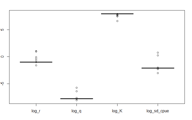
We can also visualize the jitter test using a box plot. The box plot will show if there are any odd shapes in the box plot or any outliers. A jitter test that passes a convergence check will show no odd shapes in the box plot (no quartiles) and will not have any outliers (as shown below):
# boxplots - are there any weird shapes/outliers?
boxplot(jit_res[, c(2, 4, 6, 8, 9)])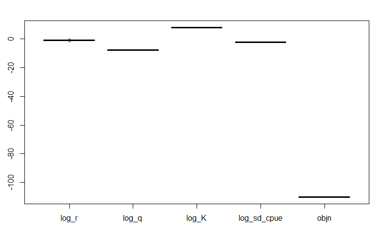
After conducting the jitter test, we can run these functions that will clean the extra ADMB files that were compiled throughout the process:
# clean extra files
clean_admb(fn = tpl_name)
if (file.exists("estpars.dat")) file.remove("estpars.dat")
if (file.exists("out.rdat")) file.remove("out.rdat")
if (file.exists("hessian.rdat")) file.remove("hessian.rdat")
if (file.exists("log_K.dat")) file.remove("log_K.dat")
if (file.exists("log_r.dat")) file.remove("log_r.dat")
if (file.exists("log_q.dat")) file.remove("log_q.dat")
if (file.exists("log_sd_cpue.dat")) file.remove("log_sd_cpue.dat")
3.6 Entire R script for the jitter test of the surplus production model
Here is the entire R script for an example of conducting a jitter test with the surplus production model.
source("base_funs.r")
source("clean_admb.r")
tpl_name <- "surp_prod_jitter"

# compile ADMB
compile_admb(fn = tpl_name, verbose = TRUE)

# set initial values and source from external files
cat("-0.6", file = "log_r.dat", sep = "\n")
cat("-3", file = "log_q.dat", sep = "\n")
cat("8", file = "log_K.dat", sep = "\n")
cat("-1", file = "log_sd_cpue.dat", sep = "\n")

# run ADMB
run_admb(fn = tpl_name, verbose = TRUE)

# get parameter estimates (used for jittering)
if (file.exists("estpars.dat")) {
  dat <- read.table("estpars.dat")
  colnames(dat) <- c("inlog_r", "log_r", "inlog_q", "log_q", "inlog_K", "log_K", "inlog_sd_cpue", "log_sd_cpue", "objn")
}

# Delete any existing version of estpars.dat
if (file.exists("estpars.dat")) file.remove("estpars.dat")

# Create header for file so we know the variables.
# sep ["\n" needed for line feed]
cat("inlog_r log_r inlogq log_q inlogK log_K inlog_sd_cpue log_sd_cpue objn", file = "estpars.dat", sep = "\n")

# Define a set of starting values
nrun <- 50 # number of reruns with new values
st_log_r <- dat$log_r + rnorm(nrun, sd = 0.1)
st_log_q <- dat$log_q + rnorm(nrun, sd = 0.1)
st_log_K <- dat$log_K + rnorm(nrun, sd = 0.1)
st_log_sd_cpue <- dat$log_sd_cpue + rnorm(nrun, sd = 0.1)

# Write out each value of the parameters and run ADMB program for each in loop
for (i in 1:length(st_log_r)) {
  cat(st_log_r[i], file = "log_r.dat", sep = "") # write one st value to file
  cat(st_log_q[i], file = "log_q.dat", sep = "") # write one st value to file
  cat(st_log_K[i], file = "log_K.dat", sep = "") # write one st value to file
  cat(st_log_sd_cpue[i], file = "log_sd_cpue.dat", sep = "") # write one st value to file
  if(Sys.info()["sysname"] == "Windows") { # windows
    system(paste0(tpl_name, ".exe"))
  } else { # most Mac's and Linux
    system(paste0("./", tpl_name))
  }
}

# read in and print results to console
jit_res <- read.table("estpars.dat", header = T)
jit_res

# boxplots - are there any weird shapes/outliers?
boxplot(jit_res[, c(2, 4, 6, 8, 9)])

# clean extra files
clean_admb(fn = tpl_name)
if (file.exists("estpars.dat")) file.remove("estpars.dat")
if (file.exists("out.rdat")) file.remove("out.rdat")
if (file.exists("hessian.rdat")) file.remove("hessian.rdat")
if (file.exists("log_K.dat")) file.remove("log_K.dat")
if (file.exists("log_r.dat")) file.remove("log_r.dat")
if (file.exists("log_q.dat")) file.remove("log_q.dat")
if (file.exists("log_sd_cpue.dat")) file.remove("log_sd_cpue.dat")
4 Jitter test interpretation
There should not be any outliers or weird shapes in the box plots. Below is an example of how the box plot would look like if the jitter test fails:
A failed jitter test is indicative that there is something wrong with the model:
Incorrect parameterization
Bad starting values (they may not make sense for the parameter)
Incorrect specification of the objective function
Incorrect equations
Data is not informative enough to estimate the parameter
This should be done for every parameter. In this tutorial, the jitter test was not conducted on \(F\) and \(sd_{catch}\). However, to fully check the convergence of this model, the jitter test should also be conducted for all estimated values of \(F\) and sensitivity analysis should be conducted on the impacts of fixing \(sd_{catch}\).