Model convergence diagnostics for non-linear models

This tutorial discusses what to check to make sure your model is consistent with convergence diagnostics. While this tutorial is focused on TMB/RTMB functions, this checklist can be applied to other non-linear models coded in other programs (e.g., ADMB).

1 Checklist:

This is a checklist of convergence checks and diagnostics that should be conducted at minimum to verify a model:

Model is executable (i.e., check objective function and gradients)
The convergence message from RTMB indicates that the diagnostics are consistent with convergence (= 0)
The Hessian matrix is positive definite
Standard errors for model estimates are reasonable
Alternative parameter starting points result in the same final parameter estimates (i.e., jitter test)
Likelihood profiles for important parameters are reasonable, e.g. (initial abundance, recruitment, natural mortality, selectivity):

It is recommended to do these checks in this order. If all of these checks pass, this indicates that the model is consistent with convergence and is estimable. It is necessary for the model to pass all these checks. If one of these checks fail, then the model is not consistent with convergence.

2 Creating the objective function in RTMB

Say you construct an objective function called obj using f as the model function and par as a list of initial parameter values. Using RTMB::MakeADFun, you can create the objective function:

obj <- RTMB::MakeADFun(f, par)

You need to check if the objective function will run before running an optimizer. You can look at this by checking if the objective function produces a likelihood and if a gradient is calculated for each parameter:

# check likelihood
obj$fn()

# check gradients
obj$gr()

What are gradients

Gradients are the partial derivatives of the objective function with respect to the model parameters (goes into one vector - obj$gr()). These partial derivatives indicate how the objective function changes (direction and magnitude) as each parameter varies. This provides information for optimization algorithms to adjust the parameters iteratively to minimize or maximize the objective function.

If the model is estimable, it will calculate a likelihood based on the initial parameters. Each parameter should also provide a gradient value. If the gradient of a parameter = 0 or NA, this means that the model is not able to estimate that parameter or the parameter is not being used in the model.

If the checks on the objective function are successful, you can run the objective function with an optimizer using the nlminb function and opt is the output:

opt <- nlminb(obj$par, obj$fn, obj$gr)

3 Convergence message

# check if the model is converged
opt$convergence
# check type of convergence
opt$message

If the diagnostics are consistent with convergence, then opt$convergence = 0. If the model did not converge, opt$convergence = 1. There can be some reasons why the model failed to converge (check opt$message for convergence message):

singular convergence: model is likely overparameterized (too complex for the data, the data does not contain enough information to estimate the parameters reliably)
false convergence: likelihood may be discontinuous (this could be related to the estimation of the parameters)

Ideally, you want the convergence message: “relative convergence”.

You may also encounter messages like these:

Warning messages:
1: In nlminb(start = par, objective = fn, gradient = gr) :
  NA/NaN function evaluation

This does not necessarily mean the model is not converged. This means that the optimizer wandered off into a bad region for a while (i.e., NAs/NaNs in the estimates) and may have gotten back out. As long as it is back in a good region by the end of the optimization, then it may be fine. However, this should be evaluated with caution, it can sometimes mean that the parameterization or model equations are not correct. Ideally, you do not want a model that is able to wander off into a bad region.

4 Hessian matrix

What is a Hessian matrix?

A Hessian matrix is a square matrix of second-order partial derivatives of the objective function. In other words, it contains information about how the rate of change of each parameter with respect to every other parameter changes.

This represents the curvature of the likelihood surface and is used to calculate estimates of uncertainty for all the estimated model parameters and chosen derived quantities.

Inverting the negative Hessian gives us the covariance matrix, which provides a measure of parameter uncertainty.
The diagonal elements of the covariance matrix (i.e., inverse of the Hessian matrix) represent the variance of individual parameters.
The square root of the diagonal elements (i.e., variance) gives standard errors of the parameter estimates.

The Hessian matrix will not be invertible if the negative log likelihood is not a true minimum. This usually occurs when the model is mis-specified, which could either mean that the model has been written incorrectly so the objective function is not differentiable/estimable with respect to all the parameters. Or the estimated parameters are confounded or overparameterized (i.e., too complex for the data). RTMB will warn you about a non-positive definite Hessian matrix.

5 Standard errors

If the standard errors for the parameter estimates are high, this suggests that the model is not fully converged. This can mean:

low precision: there is a wide range of plausible values for the parameters
lack of stability in the estimation of the parameter
overfitting: model may be too complex and is capturing noise in the data rather than true underlying patterns

Considerations to the model formulation and parameter estimates should be made if the standard errors are too high and unreasonable.

sdrep <- sdreport(obj)
sdrep

6 Jitter test

A jitter test is used to evaluate whether a model has actually converged to a global solution rather than a local minimum. This should check that none of the randomly generated starting values of the parameters results in a solution that has a smaller negative log likelihood than the reference model. A jitter test is conducted by changing the starting parameter values and rerunning the model several times. This should be done with multiple (if not all) the parameters.

# this function runs the optimizer with the new parameters (opt$par + randomization)
doone <- function() {
  fit <- nlminb(opt$par + rnorm(length(opt$par), sd = .1),
    obj$fn, obj$gr,
    control = list(eval.max = 1000, iter.max = 1000)
  )
  c(fit$par, "convergence" = fit$convergence)
}

set.seed(123456)
# jitter the parameters 100 times
jit <- replicate(100, doone())
# check if the convergence are all 0s across the 100 iterations
# check if there are any outliers or large intervals
boxplot(t(jit))

Note: the magnitude of the jittering should be done within reason (e.g., 10% CV) as extreme jitters could start the model search in an unrealistic place and then the model would not be able to detect gradients that point towards reasonable solutions.

7 Likelihood profile

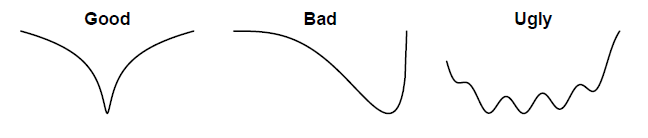
A likelihood profile shows how the negative log likelihood changes as one of the parameters is fixed across a range of values while estimating the other parameters. This helps evaluate which parameters are informative, measure the amount of information contained in the data, and check the sensitivity (i.e., the consequence of using a fixed value) of the model result to the choice of the parameters. The shape of the likelihood profile for a parameter should look like a U:

This does not have to be done on all parameters, but select important parameters. This typically includes initial abundance (e.g., R0, initial abundance at age vector), recruitment (e.g., steepness or compensation ratio), natural mortality, selectivity, etc. The goal is to identify if there are any conflicting information in the data about abundance.